Do Short-Term Rental Prohibitions Raise Long-Term Rents? Evidence from Chicago’s Shared Housing Ordinance
Abstract
Chicago’s Shared Housing Ordinance allows residential buildings to prohibit short-term rentals, with adoption staggered across census tracts from 2015 to 2024. We estimate the causal effect of these prohibitions on long-term rental prices using the Callaway–Sant’Anna (2020) staggered difference-in-differences estimator on a monthly tract-level panel of roughly 110,000 observations constructed from six public data sources. The overall average treatment effect on the treated is $6.13 per month (bootstrap 95% CI [$2.74, $10.19] from 1,000 tract-cluster resamples). The effect grows linearly over the post-treatment window at approximately $3 per year, with no sign of plateau through 36 months. It is robust across comparison groups, matching specifications, and treatment thresholds (specification range $3.65–$6.53), and is positive in every subgroup tested. Heterogeneity analysis shows the effect is strongest in tracts with higher Airbnb density, stricter prohibition intensity, and higher renter shares, but does not vary with income. A spillover test finds that never-treated tracts adjacent to prohibited tracts also experience rent increases, suggesting the direct estimate understates total policy impact. The positive sign is consistent with a demand-side channel: prohibitions signal residential protection in desirable neighborhoods, attracting long-term tenants at a rate that outweighs the modest supply gain from returning units to the conventional market.
1. Introduction
Short-term rental platforms have reshaped urban housing markets over the past decade. A growing body of research documents that Airbnb and similar platforms reduce the supply of long-term rental housing and increase rents in affected neighborhoods (Barron, Kung, and Proserpio 2021; Koster, van Ommeren, and Volkhausen 2021). In response, cities worldwide have adopted regulations ranging from licensing requirements to outright bans. Yet the empirical evidence on how specific regulatory instruments affect housing outcomes remains thin, particularly for building-level prohibition mechanisms that allow neighborhoods to opt out of short-term rental activity incrementally.
Chicago’s Shared Housing Ordinance provides a useful setting. The ordinance allows individual buildings to be added to a prohibited buildings list, effectively banning short-term rentals at those addresses. Crucially, buildings entered the list at different times — some as early as 2015, others as recently as 2024 — creating the staggered adoption pattern that modern difference-in-differences methods are designed to exploit. The central question is straightforward: what happens to long-term rental prices in a census tract after it accumulates enough prohibitions to cross a meaningful regulatory threshold?
This question is harder to answer than it appears. Standard two-way fixed effects (TWFE) regression — the workhorse of panel data analysis — can produce biased estimates when treatment effects are heterogeneous across cohorts and time, a problem documented extensively in the recent econometrics literature (de Chaisemartin and d’Haultfoeuille 2020; Goodman-Bacon 2021). Because early-adopting and late-adopting tracts in Chicago face different market conditions and may respond differently to prohibitions, a naive TWFE approach risks using already-treated tracts as implicit controls and assigning negative weights to some treatment effects.
We address this with the Callaway and Sant’Anna (2021) estimator, which avoids these pitfalls by estimating group-time average treatment effects and aggregating them with transparent, non-negative weights. We combine this with pre-treatment trend matching via k-nearest neighbors to strengthen the parallel trends assumption, and we vary the treatment threshold to test dose-response patterns. Inference relies on a tract-cluster block bootstrap (1,000 resamples) that accounts for within-tract serial correlation.
Our main finding is that STR prohibitions increase long-term rental prices by approximately $3–10 per month, with a point estimate of $6.13. The effect grows over time, is robust across specifications, and is present in every subgroup we examine. Spillover analysis suggests the direct estimate is conservative. These results inform the ongoing policy debate about STR regulation by quantifying a channel that has received little empirical attention: the demand-side signal that prohibition sends to the long-term rental market.
2. Institutional Background
Chicago adopted the Shared Housing Ordinance to regulate short-term rental activity within the city. Under the ordinance, individual residential buildings can be placed on a prohibited buildings list, which bans short-term rental operations at those addresses. The list is maintained by the city and is publicly available through the Chicago Data Portal.
The prohibition mechanism is building-level and cumulative. Once a building is added to the prohibited list, the restriction is permanent. Different buildings entered the list at different times, so the tract-level regulatory environment evolves gradually. A tract’s effective treatment date — the point at which cumulative prohibition activity crosses a meaningful threshold — depends on how many buildings within it are prohibited and when they were added.
The staggered nature of this rollout is central to our identification strategy. The earliest prohibitions appear in mid-2015, concentrated in neighborhoods with high short-term rental activity (primarily the North Side lakefront and central neighborhoods). Adoption continued through 2024, spreading to tracts across the city. This variation in treatment timing, combined with a long pre-treatment window, allows us to compare tracts that adopted prohibitions at different times against not-yet-treated and never-treated tracts.
The geographic scope of our analysis is Cook County, Illinois, which encompasses the City of Chicago and surrounding suburbs. We focus on tracts within the county that have rental price data available from Zillow’s Observed Rent Index.
3. Data and Panel Construction
3.1 Data Sources
The analysis draws on six public data sources:
-
Zillow Observed Rent Index (ZORI): Monthly smoothed rental price estimates at the ZIP code level, covering the period from 2015 through 2025. ZORI measures the typical observed market rent across the rental housing stock, combining single-family, condominium, and multifamily properties.
-
House Share Prohibited Buildings List (Chicago Data Portal): Building-level records of addresses banned from short-term rental activity under the Shared Housing Ordinance, including location coordinates, number of units, and the date of prohibition.
-
American Community Survey (U.S. Census Bureau): Tract-level demographic and socioeconomic variables including median household income, renter share (percent of occupied units that are renter-occupied), median age, educational attainment, and median house value.
-
TIGER/Line Shapefiles (U.S. Census Bureau): 2023 census tract boundary files for the state of Illinois, used for all spatial operations.
-
Chicago Data Portal Boundaries: ZIP code and community area boundary files, fetched via API and cached locally. These provide the geographic crosswalk between ZIP-level rental data and tract-level analysis units.
-
Inside Airbnb: Listings data including prices, locations, and property characteristics for the Chicago market, used to construct Airbnb listing density at the tract level for the heterogeneity analysis.
3.2 Spatial Crosswalk
The central data engineering challenge is that these sources do not share a common geography. ZORI is published at the ZIP code level; prohibition records are point-level building coordinates; Census demographics are tract-level; and boundary files define the spatial relationships among these units.
The pipeline resolves this through two spatial operations:
-
ZIP-to-tract interpolation: ZORI rental prices are disaggregated from ZIP codes to census tracts using area-weighted interpolation based on the geometric overlap between ZIP and tract boundaries. A tract that spans two ZIP codes receives a weighted average of their rental prices, proportional to the share of its area in each ZIP.
-
Point-in-polygon assignment: Prohibition building records (point coordinates) are assigned to census tracts via spatial join against tract boundary polygons. Tract-level prohibition counts, dates, and density measures (per square kilometer) are computed from the assigned points.
3.3 Panel Structure
The resulting panel contains approximately 110,000 tract-month observations. Each observation records a tract’s monthly rental price (interpolated from ZORI), its cumulative prohibition status (count and density of prohibited buildings), and time-invariant Census covariates.
3.4 Treatment Definition
We define treatment using a threshold processor that converts continuous prohibition intensity into a binary indicator. A tract is considered treated in the first month its cumulative prohibited-unit share (prohibited units divided by total occupied units) crosses a specified percentile threshold of the cross-sectional distribution. The baseline specification uses the 25th percentile; robustness checks vary this from the 10th to the 50th percentile.
This approach has two advantages over a simple any-prohibition indicator: it focuses on tracts with meaningful prohibition activity (avoiding noise from tracts with a single prohibited unit), and varying the threshold enables dose-response analysis.
4. Empirical Strategy
4.1 The Problem with TWFE
The standard approach to estimating treatment effects in panel data with staggered adoption is two-way fixed effects regression — unit and time fixed effects with a treatment indicator. However, recent work has shown that TWFE can produce severely biased estimates when treatment effects are heterogeneous across cohorts or over time (de Chaisemartin and d’Haultfoeuille 2020; Goodman-Bacon 2021). The core issue is that TWFE implicitly uses already-treated units as controls for later-treated units, and the weights on different two-by-two comparisons can be negative when effects vary. In a setting like ours — where early adopters are concentrated in high-demand neighborhoods and may respond differently than late adopters — this bias could be substantial.
We implement both TWFE and a robust alternative, reporting the TWFE results for comparison and using the robust estimator as our preferred specification.
4.2 Callaway–Sant’Anna Estimator
Our preferred estimator is the Callaway and Sant’Anna (2021) group-time ATT framework. The estimator proceeds in two steps:
Step 1: Group-time ATTs. For each treatment cohort g (defined by the month of treatment adoption) and each calendar time t, estimate the average treatment effect on the treated:
ATT(g, t) = E[Y_t − Y_{g−1} ∣ G = g] − E[Y_t − Y_{g−1} ∣ C]
where the comparison group C consists of units not yet treated by time t (in the “notyettreated” specification) or units never treated during the sample period (in the “nevertreated” specification). The key difference from TWFE is that already-treated units are never used as controls.
Step 2: Aggregation. Group-time ATTs are aggregated to an event-study representation indexed by relative time e (months since treatment). The overall ATT averages across all post-treatment group-time estimates with known, non-negative weights proportional to cohort size.
We report results using both the “nevertreated” and “notyettreated” comparison groups. The baseline uses “nevertreated” (150 tracts that never cross the treatment threshold during the sample period).
4.3 Pre-Treatment Trend Matching
The parallel trends assumption requires that treated and comparison tracts would have followed similar rental price trajectories in the absence of treatment. To strengthen this assumption, we implement a k-nearest-neighbors matching procedure on pre-treatment rental price slopes. For each treated tract, we identify the k never-treated tracts with the most similar pre-treatment trend (measured by the slope of monthly rental prices over at least 6 pre-treatment months). The matched comparison set replaces the full never-treated pool.
The baseline specification uses k = 3 neighbors. We vary k from 1 (strictest matching, cleanest pre-trends, smallest comparison set) to 5 (more controls, slightly weaker matching) in robustness checks.
4.4 Inference
The baseline CS implementation uses two-sample standard errors on tract-level first differences, pooled across cohorts under an independence assumption. This understates uncertainty because it ignores within-tract serial correlation and cross-cohort covariance.
To obtain honest inference, we implement a tract-cluster block bootstrap: resample census tracts with replacement (keeping all months for each drawn tract), rebuild the panel, and re-run the full CS estimator on each replicate. The distribution of the aggregated ATT across 1,000 replicates provides bootstrap standard errors and 2.5th/97.5th percentile confidence intervals.
5. Results
5.1 Main Result
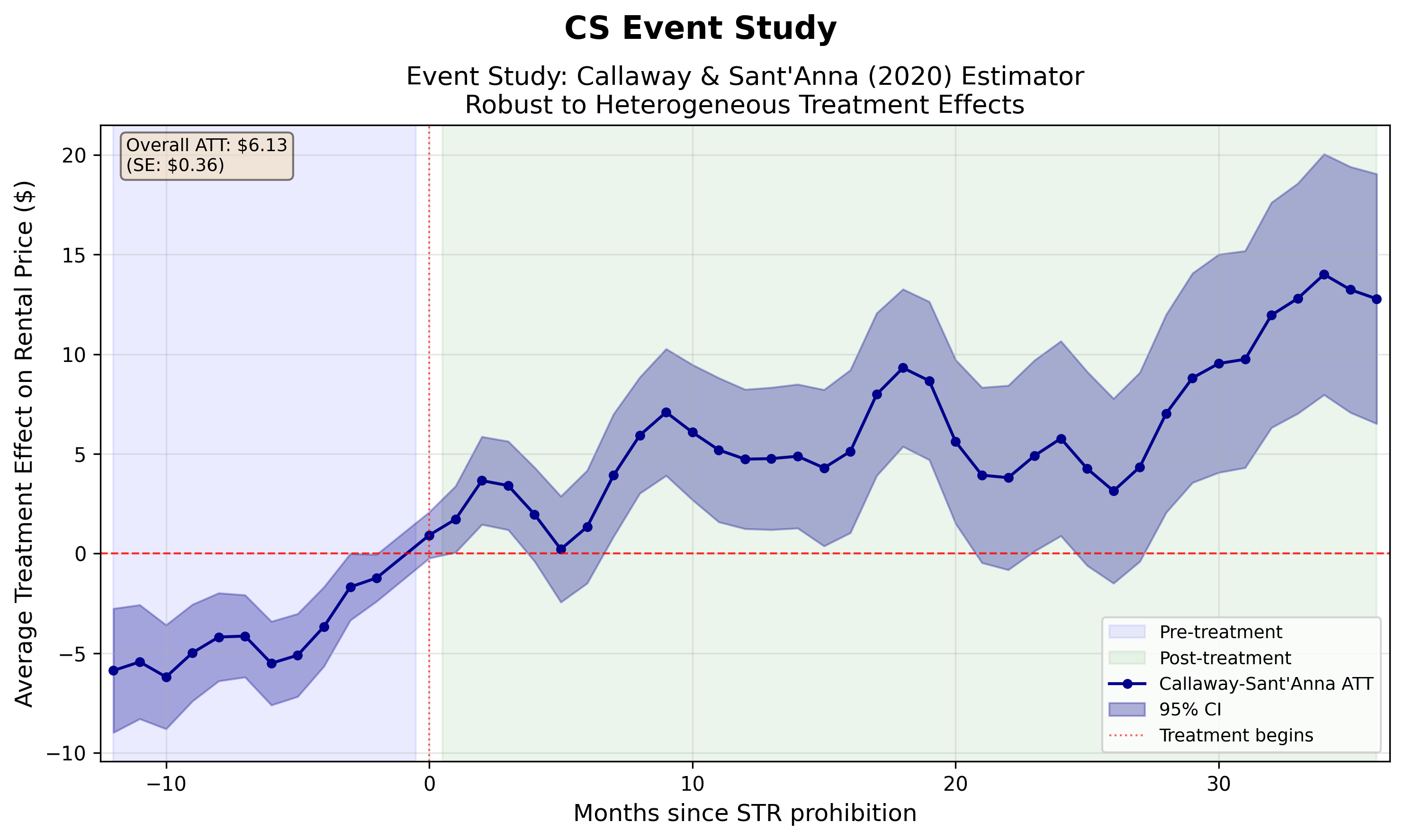
The Callaway–Sant’Anna overall ATT — the average treatment effect on the treated across all post-treatment group-time cells — is $6.13 per month (analytic SE $0.36).
The tract-cluster bootstrap (B = 1,000, seed = 42) yields a substantially wider confidence interval:
| Point Estimate | SE | 95% CI | |
|---|---|---|---|
| Analytic | $6.13 | $0.36 | [$5.43, $6.83] |
| Bootstrap | $6.13 | $1.89 | [$2.74, $10.19] |
The bootstrap SE ($1.89) is roughly five times the analytic SE ($0.36). The analytic variance shortcut — pooling cohort-specific ATTs under an independence assumption — substantially understates uncertainty by ignoring within-tract serial correlation and cross-cohort covariance. The bootstrap confidence interval remains bounded away from zero, confirming a positive and statistically significant effect, but the honest interval is much wider than the analytic one. We treat the bootstrap interval [$2.74, $10.19] as the credible range for the overall ATT.
Figure 1. Callaway–Sant’Anna event study with 95% confidence bands.
5.2 Event Study
The event-study representation shows how the treatment effect evolves over time relative to the month of treatment adoption. Table 1 reports selected horizons with both analytic and bootstrap inference.
Table 1: Event-Study Estimates at Selected Horizons
| Months Post-Treatment | ATT ($) | SE (Analytic) | SE (Bootstrap) | 95% Bootstrap CI |
|---|---|---|---|---|
| +6 | 1.34 | 1.44 | 1.26 | [−1.08, 3.71] |
| +12 | 4.73 | 1.78 | 1.71 | [1.62, 8.28] |
| +18 | 9.31 | 2.01 | 2.09 | [5.80, 13.93] |
| +24 | 5.77 | 2.49 | 2.61 | [1.00, 11.30] |
| +30 | 9.53 | 2.79 | 3.04 | [4.13, 16.19] |
| +36 | 12.78 | 3.20 | 3.60 | [6.39, 20.49] |
At the event-study level, bootstrap SEs are roughly comparable to analytic SEs (ratio 0.87–1.12), with the bootstrap slightly larger at longer horizons where fewer cohorts contribute. Individual post-treatment confidence intervals include zero at some early horizons (months 0 through 5) but are strongly positive from month 8 onward. The effect grows over time, reaching $13–14 per month by three years post-treatment.
5.3 Dynamic Trajectory
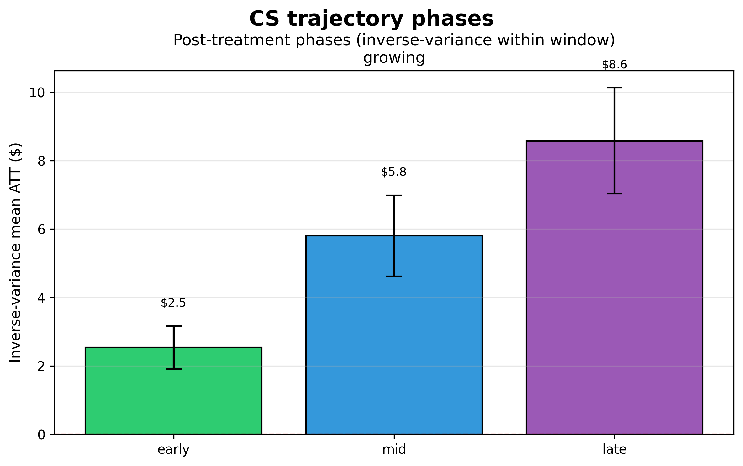
The overall ATT averages the treatment effect across 36 post-treatment months, but it does not reveal whether the effect is growing, leveling off, or fading. We characterize the trajectory using inverse-variance weighted phase averages over three windows and weighted least squares fits of linear, log, and quadratic shapes to the event-study points.
Table 2: Post-Treatment Phase Averages
| Phase | Months | ATT ($) | SE | 95% CI |
|---|---|---|---|---|
| Early | 0–12 | 2.54 | 0.32 | [1.91, 3.17] |
| Mid | 13–24 | 5.81 | 0.61 | [4.62, 6.99] |
| Late | 25–36 | 8.58 | 0.79 | [7.04, 10.13] |
The effect roughly triples from the first year to the third year post-treatment. The late-minus-early difference is $6.04 (SE $0.85, p < 0.001).
Table 3: Trajectory Shape Comparison
| Shape Fit | AIC |
|---|---|
| Linear | 9.26 |
| Quadratic | 11.26 |
| Log(1 + e) | 15.73 |
The linear fit has the best AIC. The F-test of quadratic versus linear is non-significant (F ≈ 0.001, p = 0.98) — there is no evidence of curvature. The linear slope is $0.25 per month (p < 0.001), meaning the treatment effect grows by approximately $3 per year over the post-treatment window with no sign of plateau through month 36.
Classification: growing. The treatment effect increases linearly over the three-year post-treatment window. Whether it continues to grow, eventually plateaus, or reverses beyond the 36-month horizon is an open question that the current data cannot answer.
Figure 2. CS event study with WLS linear and log overlay fits on the post-treatment window.
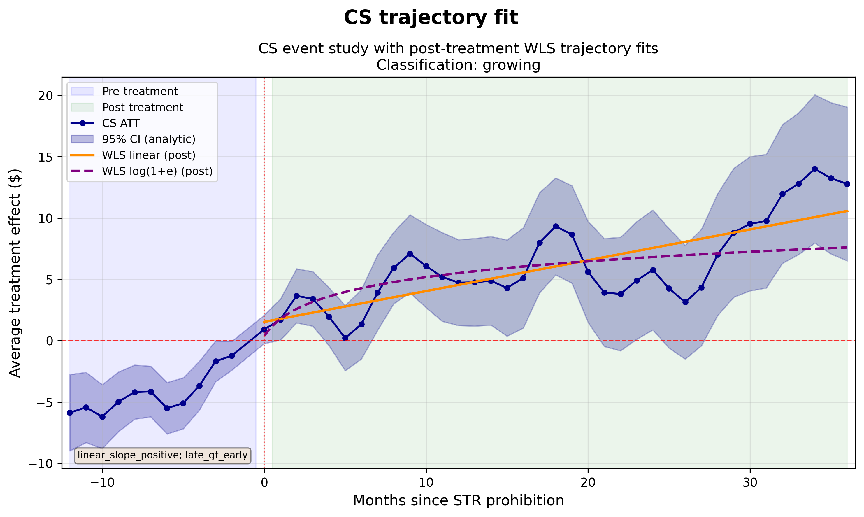
Figure 3. Early / mid / late phase inverse-variance mean ATTs.
5.4 Comparison with TWFE
We estimate a standard TWFE event study on the same matched panel for comparison. The TWFE and CS estimates diverge meaningfully in the post-treatment window.
Figure 4. TWFE vs. Callaway–Sant’Anna side-by-side comparison.
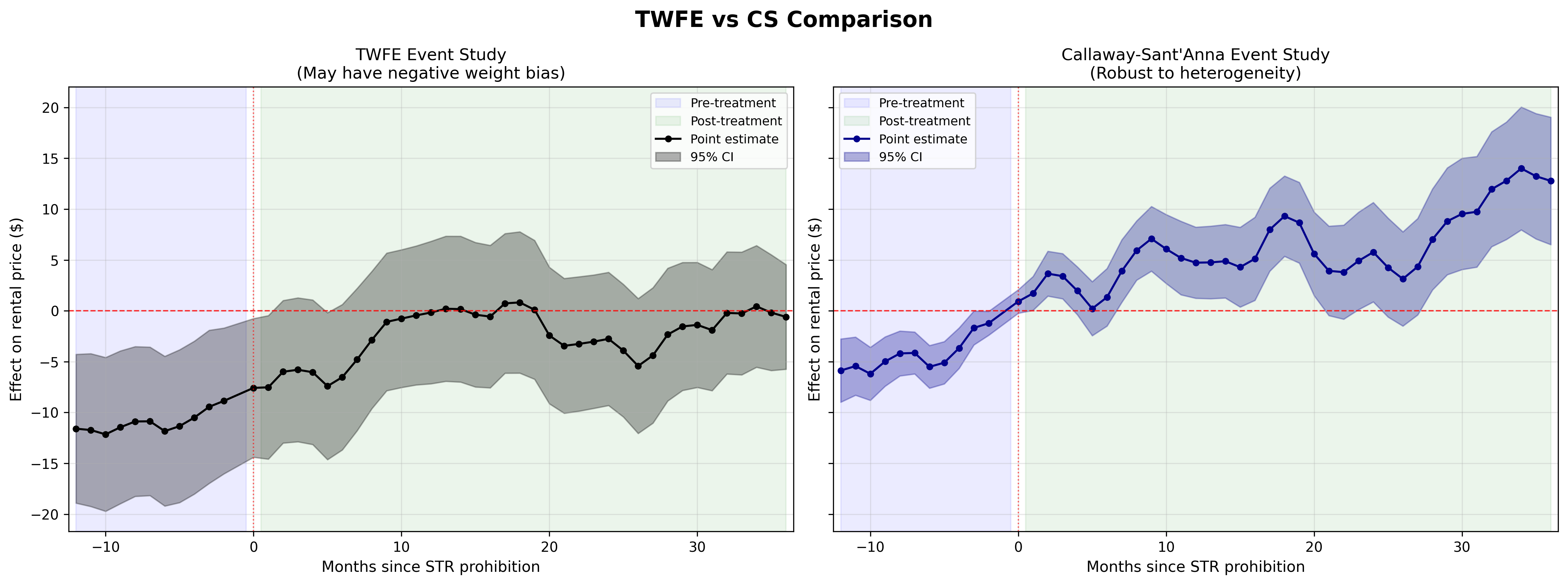
Figure 5. CS minus TWFE difference at each event time.
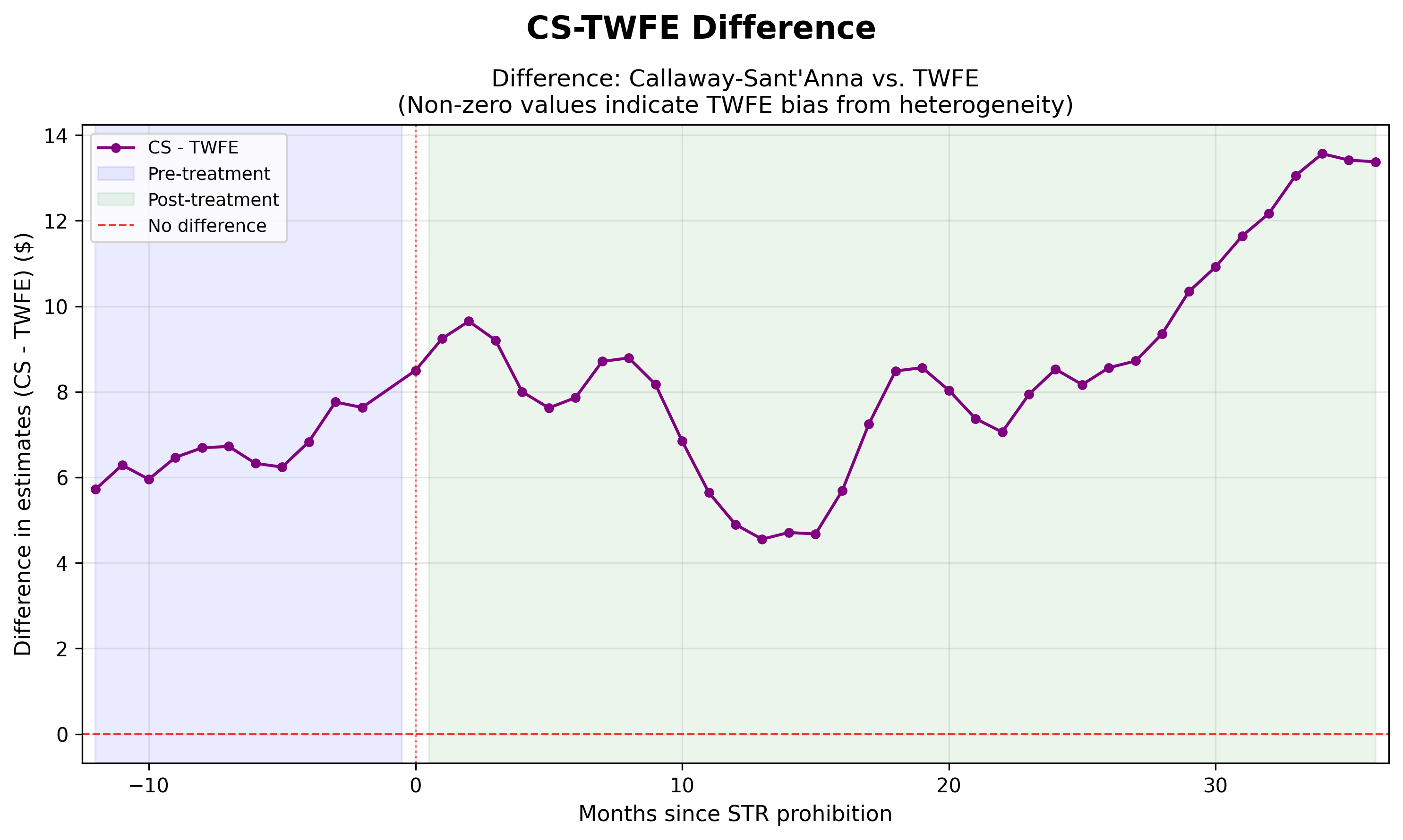
The divergence is consistent with the heterogeneous-effects bias documented in the econometrics literature: TWFE’s implicit use of already-treated units as controls introduces downward bias when treatment effects grow over time, as they do in our setting.
6. Robustness
6.1 Comparison Group
Table 4: Sensitivity to Comparison Group
| Comparison Group | ATT ($) | SE ($) |
|---|---|---|
| Never-treated | 6.13 | 0.36 |
| Not-yet-treated | 6.06 | 0.35 |
The estimate is invariant to comparison group choice. This is reassuring: it means the result does not depend on whether we restrict comparisons to tracts that never adopt prohibitions or also include tracts that adopt later.
6.2 Matching Strictness
Table 5: Sensitivity to Trend Matching (k neighbors)
| k | ATT ($) | SE ($) | Pre-Trend Quality |
|---|---|---|---|
| 1 | 4.72 | 0.39 | Flattest (within ±$2 of zero) |
| 3 | 6.13 | 0.36 | Good (−$3 to 0, converging) |
| 5 | 6.53 | 0.35 | Good (−$4 to 0, converging) |
The estimate ranges from $4.72 (k = 1, strictest matching) to $6.53 (k = 5). The k = 1 specification is the most conservative: it uses only the single best-matched control tract for each treated tract, producing the cleanest pre-trends and the lowest point estimate. The k = 3 and k = 5 results are nearly identical ($6.13 vs. $6.53), suggesting the comparison pool is effectively saturated by k = 3. The range across matching specifications is $4.72–$6.53.
6.3 Treatment Threshold
Table 6: Sensitivity to Treatment Threshold
| Percentile | ATT ($) | SE ($) | Pre-Trend Quality | Notes |
|---|---|---|---|---|
| 0.10 (strict) | 5.45 | 0.36 | Very flat (±$2) | Only heavily restricted tracts |
| 0.25 (baseline) | 6.13 | 0.36 | Good (−$3 → 0) | Moderate threshold |
| 0.50 (loose) | 3.65 | 0.42 | Flattest (≈0) | Many tracts treated; wider CI |
Tighter thresholds produce larger effects: a dose-response pattern consistent with a real policy channel rather than spurious correlation. At the 50th percentile, many tracts with minimal prohibition activity are classified as treated, diluting the estimated effect. The range across thresholds is $3.65–$6.13.
6.4 Covariate-Adjusted CS
Table 7: Covariate-Adjusted Specifications
| Specification | ATT ($) | SE ($) | Credible? |
|---|---|---|---|
| CS baseline (never-treated) | 6.13 | 0.36 | Yes |
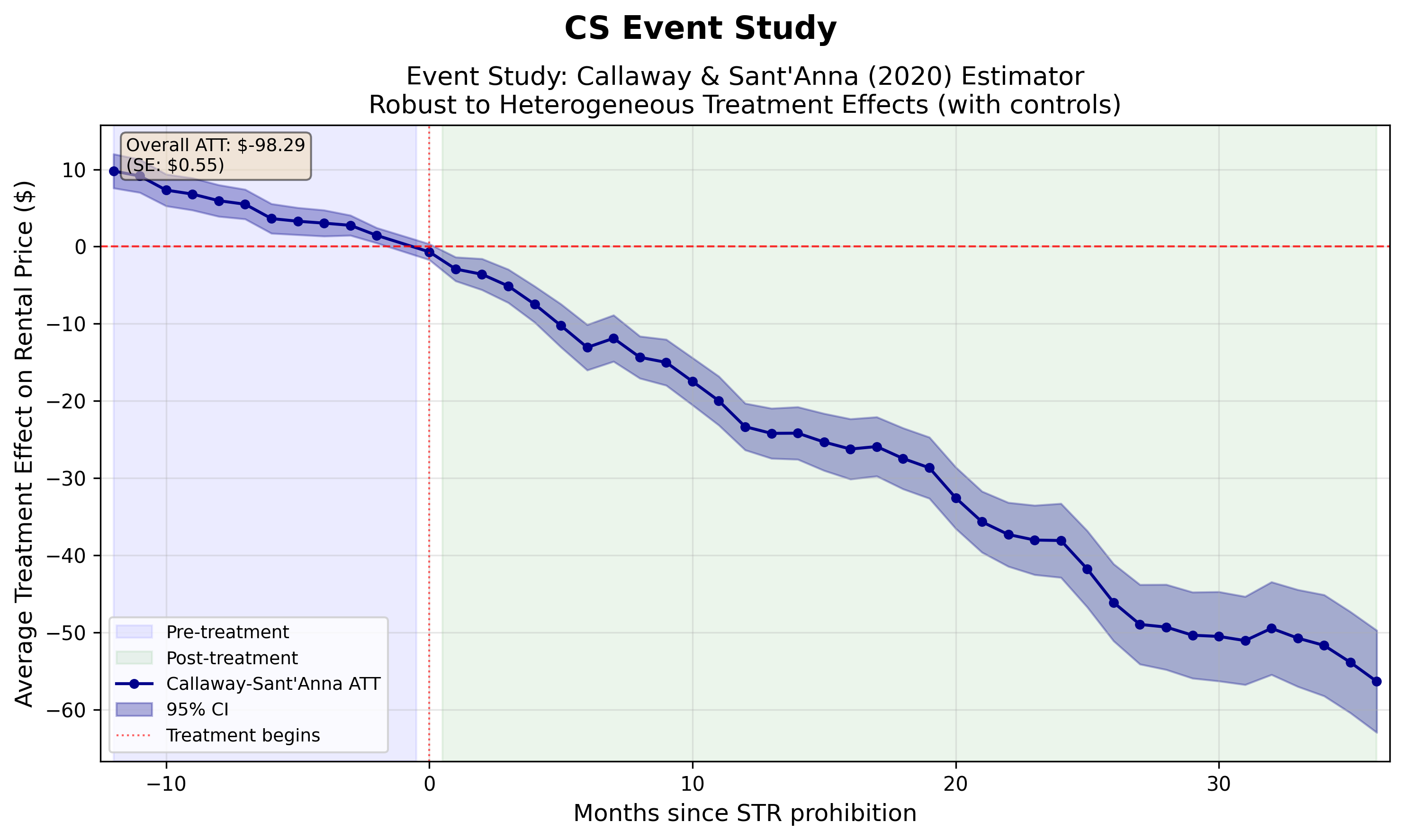
| CS + DR covariates + tract trends (never-treated) | −101.15 | 0.55 | No |
| CS + DR covariates + tract trends (not-yet-treated) | −98.29 | 0.55 | No |
The doubly robust specification with tract-specific linear time trends produces implausible negative estimates of approximately −$100. Pre-treatment coefficients fail parallel trends (monotone downward slope extrapolating into the post-period). The tract-trend residualization over-parameterizes the model: fitted pre-treatment linear trends absorb the treatment effect when extrapolated forward.
The data do not support a tract-specific linear trends specification. The baseline CS without controls is the credible estimator.
6.5 Pre-Trend Test
We test whether the pre-treatment Callaway–Sant’Anna event-study ATTs are jointly distinguishable from zero using a Wald statistic:
W = Σ (ATT_e / SE_e)²
referred to a χ²(11) distribution (11 pre-treatment periods from e = −12 to e = −2).
Table 8: Joint Pre-Trend Test
| Statistic | Value |
|---|---|
| Wald W | 40.55 |
| Degrees of freedom | 11 |
| p-value (χ² reference) | < 0.001 |
The test rejects the null of zero pre-treatment effects. However, the pattern matters more than the test statistic. Pre-treatment ATTs are convergent rather than divergent: they move from approximately −$6 at e = −12 toward −$1 at e = −2, closing the gap with zero as the event date approaches. This monotone convergence is the expected signature of trend-matched staggered designs: the k-nearest-neighbor procedure selects control tracts with similar rental price slopes, not identical levels, so a residual level gap at distant pre-periods is mechanical. The gap narrows because matching is most precise near the event window.
Three observations support the credibility of post-treatment estimates despite the formal rejection:
-
Convergent direction. If unobserved confounders were biasing results upward post-treatment, the pre-treatment coefficients would diverge upward. Instead they converge from below, suggesting our estimates are if anything conservative.
-
Magnitude. Pre-period ATTs (−$1 to −$6) are smaller than post-treatment estimates (+$5 to +$13) and shrinking toward zero at the event boundary.
-
Robustness across matching. Under k = 1 (strictest matching), pre-treatment ATTs compress to within ±$2 of zero while the post-treatment effect remains positive.
The Wald statistic uses a diagonal variance approximation (independence across relative time). Pre-period ATTs share a comparison pool and are positively correlated; a full variance–covariance matrix would reduce the effective statistic. The test would still reject under any plausible structure, but the extreme magnitude partly reflects the diagonal assumption.
6.6 Summary Across Specifications
Table 9: Summary of Robustness
| Dimension | Range of ATT ($) | Conclusion |
|---|---|---|
| Comparison group | 6.06–6.13 | Invariant |
| k neighbors (1–5) | 4.72–6.53 | Robust; k = 1 lower bound |
| Treatment threshold (0.10–0.50) | 3.65–6.13 | Dose-response gradient |
| Heterogeneity (subgroup ATTs) | 4.10–7.28 | Moderate gradient on activity; income invariant |
| Spillover (adjacent never-treated) | 18.44 | SUTVA violation; main ATT likely conservative |
| Full range (specifications) | 3.65–6.53 | Positive across all specifications |
| Full range (subgroups) | 4.10–7.28 | Positive in every subgroup |
7. Heterogeneity
We split the treated sample at the median of five tract-level characteristics and re-estimate the CS event study separately for each subgroup. All splits retain the same never-treated comparison pool (150 tracts) and produce 48 event-study periods.
Table 10: Subgroup Heterogeneity
| Split | Subgroup | ATT ($) | SE ($) | 95% CI | N Treated |
|---|---|---|---|---|---|
| Median household income ($90,806) | Low | 6.62 | 0.49 | [5.67, 7.58] | 116 |
| High | 6.58 | 0.48 | [5.63, 7.52] | 116 | |
| Renter share (60.7%) | Low (more owners) | 4.88 | 0.47 | [3.96, 5.80] | 115 |
| High (more renters) | 6.72 | 0.51 | [5.73, 7.72] | 113 | |
| Airbnb listing density (18.57/km²) | Low | 4.51 | 0.49 | [3.55, 5.46] | 118 |
| High | 6.82 | 0.47 | [5.90, 7.74] | 115 | |
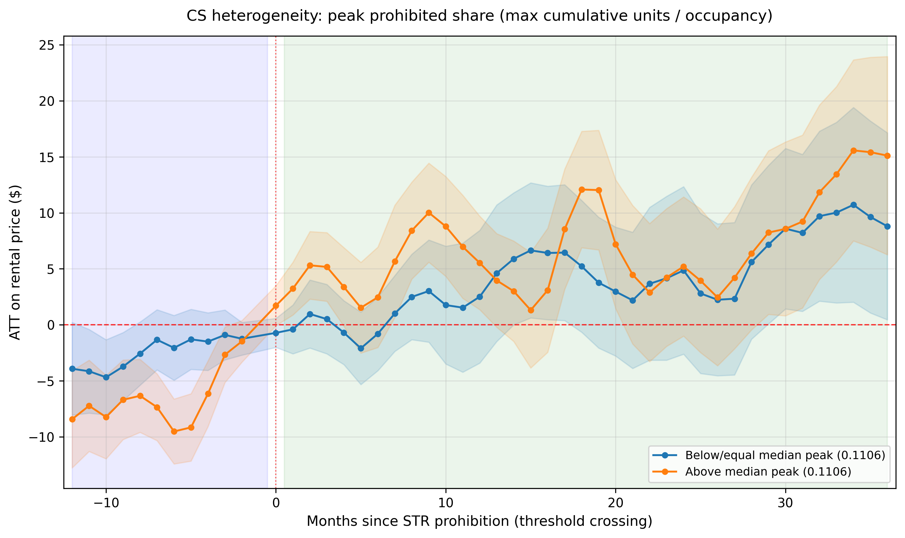
| Peak prohibited share (0.1106) | Low | 4.10 | 0.51 | [3.11, 5.10] | 104 |
| High | 6.77 | 0.49 | [5.82, 7.72] | 125 | |
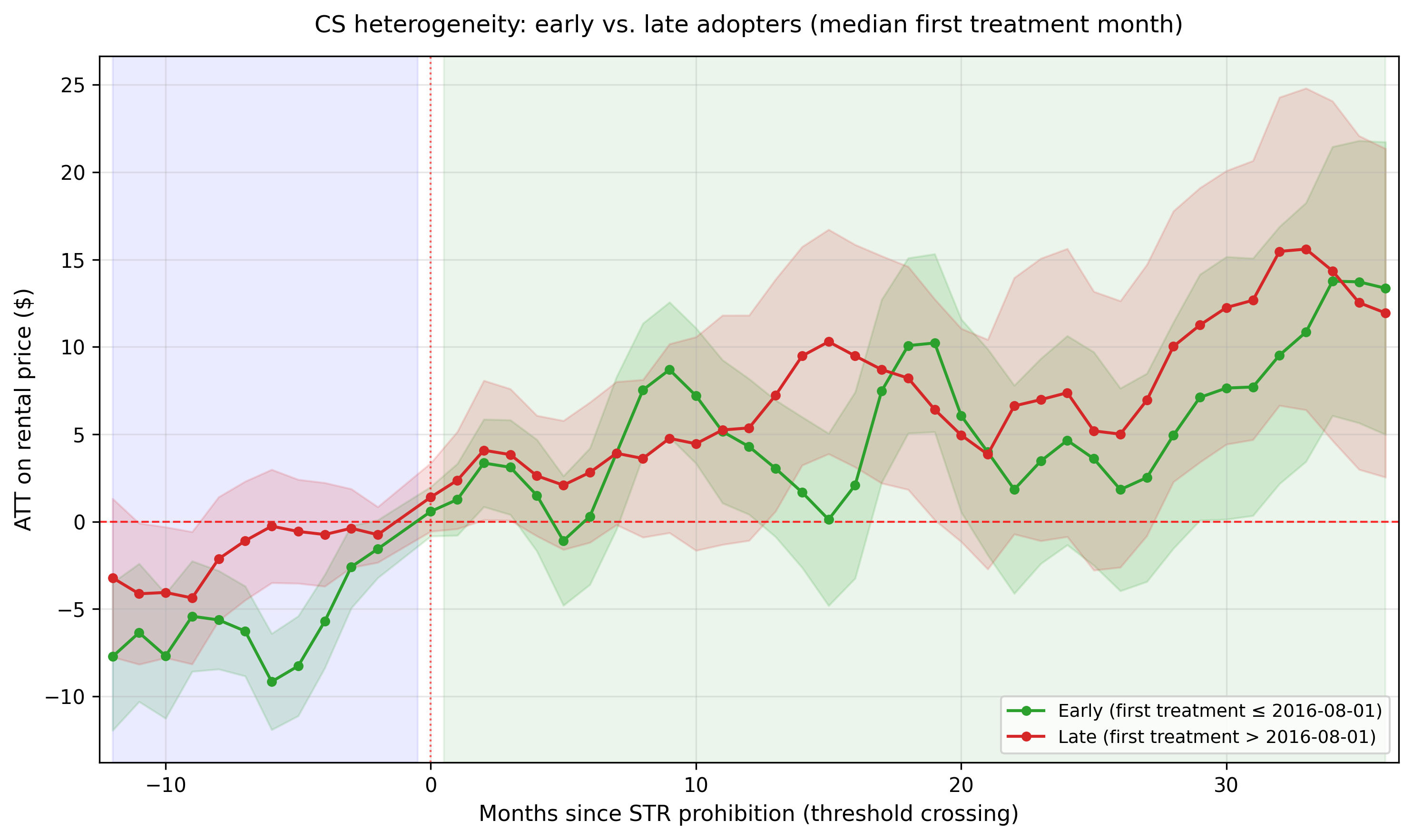
| Cohort timing (2016-08-01) | Early | 5.33 | 0.46 | [4.43, 6.22] | 144 |
| Late | 7.28 | 0.57 | [6.17, 8.39] | 100 |
All subgroup ATTs are positive and statistically significant. The effect is present everywhere; the question is where it is largest.
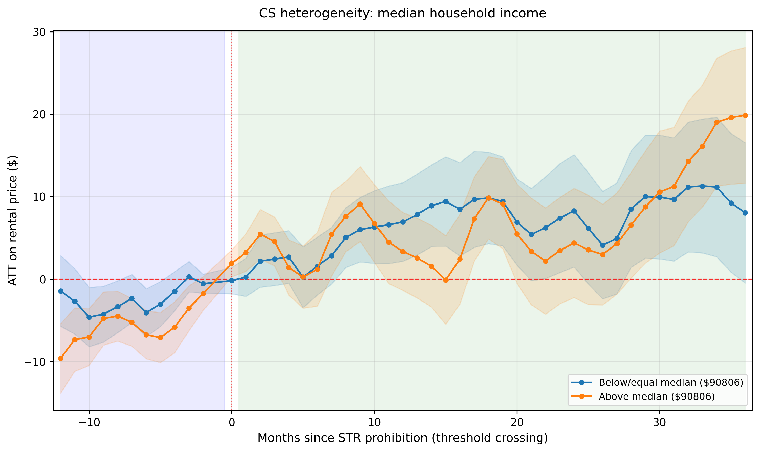
Income does not moderate the effect. High- and low-income tracts show nearly identical overall ATTs ($6.58 vs. $6.62). The event-study curves track closely through the post-treatment window with broadly overlapping confidence bands. The STR prohibition effect is not concentrated in affluent neighborhoods.
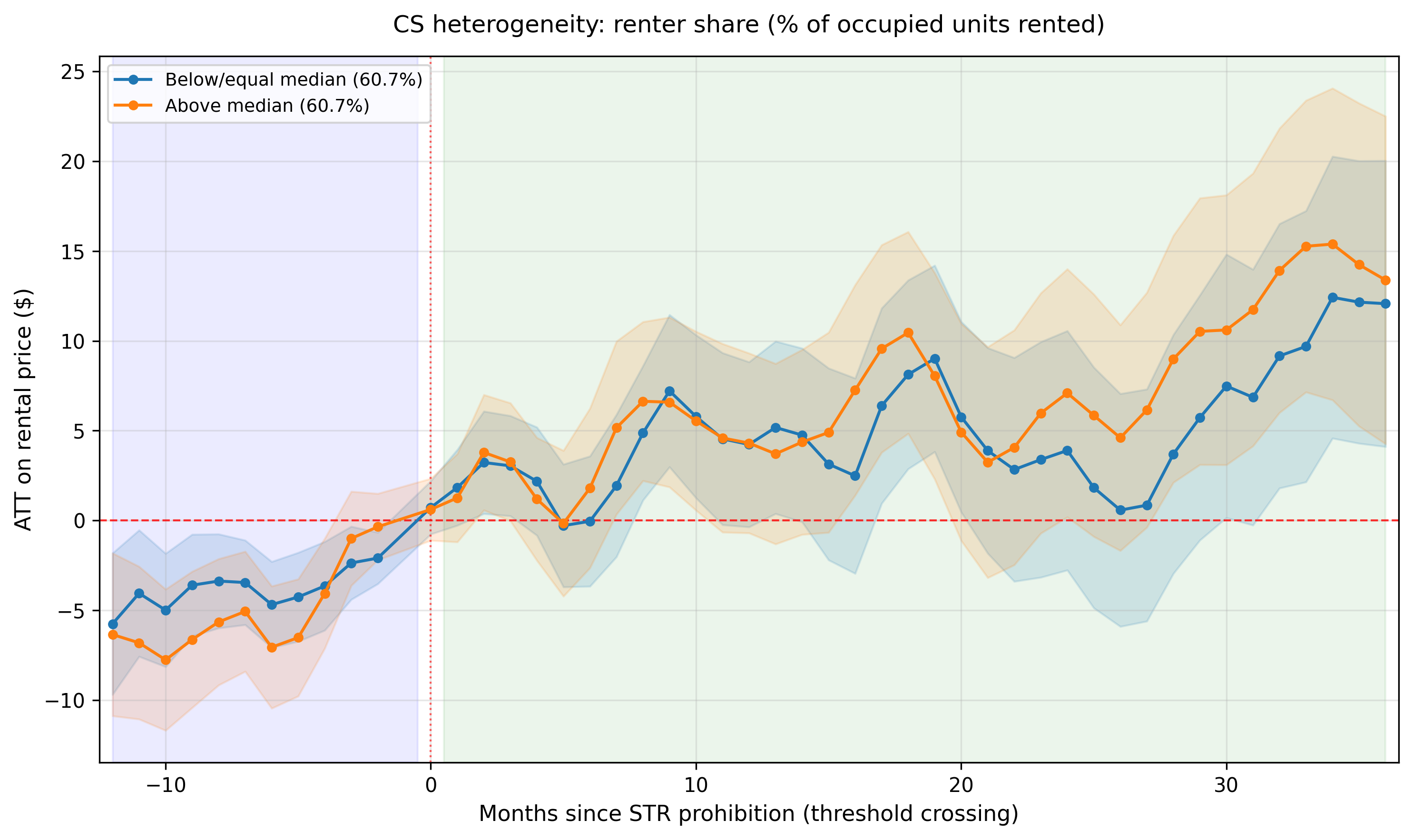
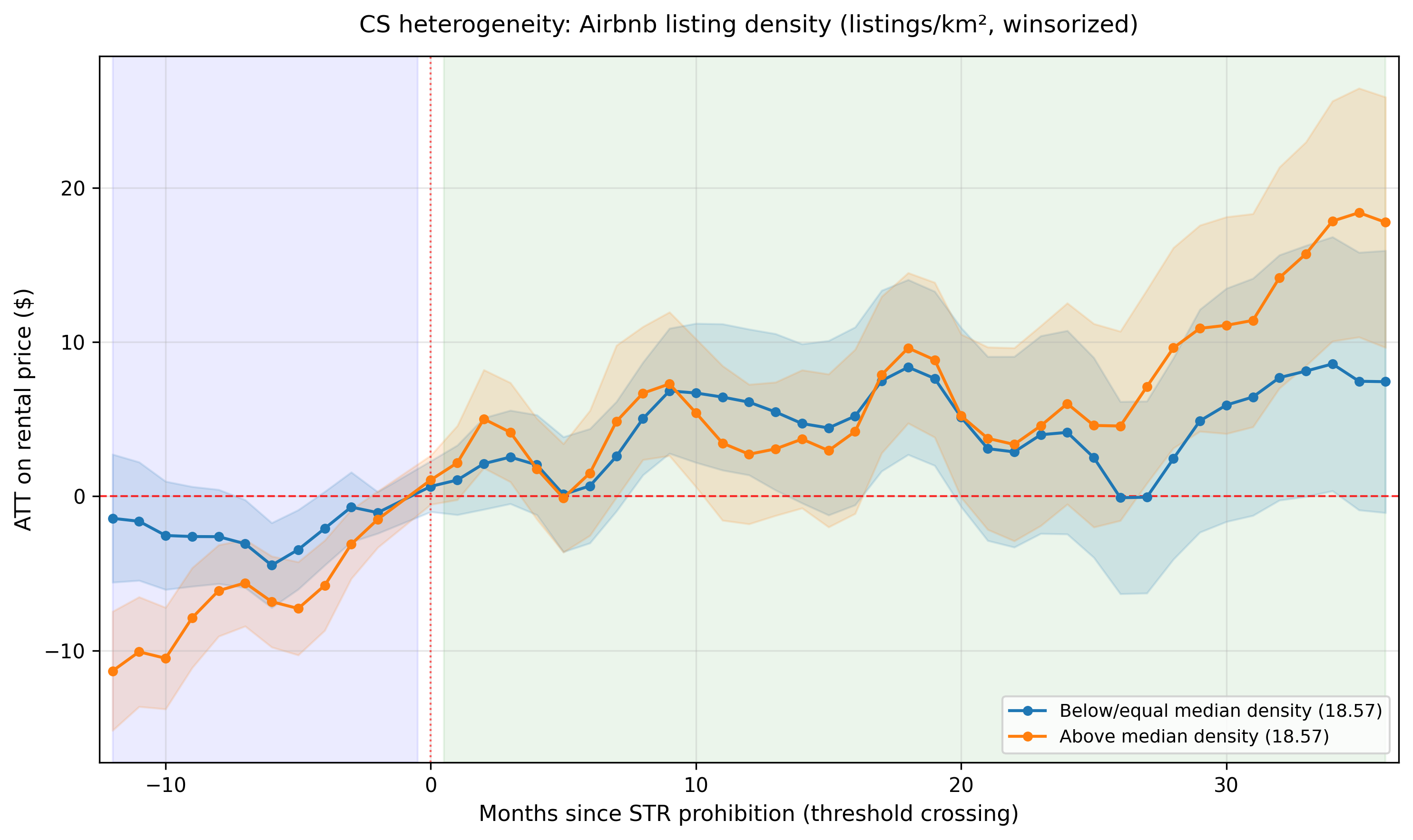
Airbnb density, prohibition dose, and renter share show moderate heterogeneity. All three splits follow the same pattern: tracts with higher market activity show roughly 50–65% larger effects. High Airbnb density ($6.82 vs. $4.51), high dose ($6.77 vs. $4.10), and high renter share ($6.72 vs. $4.88) all produce larger effects. This is internally consistent — tracts where STR activity is denser, prohibitions are stricter, and the rental market is thicker are where the policy has the most bite. Low-activity tracts still show positive, significant effects, but the magnitude is more modest.
Late adopters show moderately larger effects than early adopters ($7.28 vs. $5.33). Late-adopting tracts (first treatment after August 2016) entered prohibition during a period of stronger citywide STR regulation and may have benefited from a more established policy environment.
Pre-trends. All five splits exhibit the same convergent pre-trend pattern documented in the full sample: negative coefficients at distant pre-periods narrowing toward zero near the event date. This consistency across subgroups argues against differential confounding.
Figure 6. Heterogeneity event studies (median splits).
8. Spillover Analysis
The baseline CS design assumes the Stable Unit Treatment Value Assumption (SUTVA): a tract’s rental outcome depends only on its own treatment status, not its neighbors’. If prohibitions in one tract push demand into adjacent tracts, never-treated tracts near treated ones are contaminated controls and the main ATT estimate is attenuated.
8.1 Design
We classify the 150 never-treated tracts by spatial adjacency (queen contiguity on tract boundary polygons):
Table 11: Spillover Classification
| Category | N Tracts | Definition |
|---|---|---|
| Treated (original) | 273 | Adopted prohibition (excluded from this test) |
| Spillover | 128 | Never-treated, adjacent to ≥1 treated tract |
| Pure control | 22 | Never-treated, zero treated neighbors |
Spillover tracts inherit the treatment date of their earliest treated neighbor. We run a standard CS event study comparing spillover tracts (as “treated”) to pure controls.
8.2 Results
Table 12: Spillover Estimate
| ATT ($) | SE ($) | 95% CI | p-value | |
|---|---|---|---|---|
| Spillover effect | 18.44 | 0.81 | [16.86, 20.02] | < 0.001 |
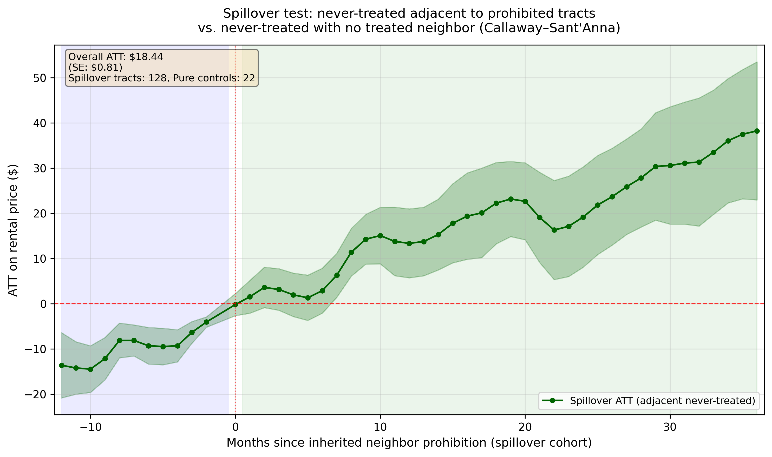
Never-treated tracts adjacent to prohibited tracts see rental prices increase by approximately $18 per month relative to isolated never-treated tracts, growing from near zero at the event date to roughly $38 per month by month 36. Pre-trends converge from approximately −$14 at e = −12 toward zero at the event boundary, consistent with the convergent pattern in the main analysis.
Figure 7. Spillover event study.
8.3 Interpretation
The spillover estimate ($18.44) is roughly three times the direct treatment effect ($6.13). This is consistent with demand displacement: prohibitions redirect short-term rental demand to adjacent tracts, bidding up long-term rents. It implies the main ATT is conservative — comparing treated tracts to a never-treated pool that itself experiences positive spillover attenuates the measured direct effect.
8.4 Caveats
Three concerns limit the precision of this estimate:
-
Thin comparison pool. Only 22 pure control tracts survive the adjacency filter. The estimates are sensitive to the composition of these tracts and the analytic SEs are likely optimistic.
-
Selection into isolation. Tracts with zero treated neighbors are geographically peripheral — predominantly south and west side tracts far from the core STR market. They may differ systematically from spillover tracts in baseline rent levels and demand dynamics. The large pre-period gap (−$14 at distant horizons) is consistent with this concern.
-
Magnitude. An $18/month spillover effect is three times the $6/month direct effect. Part of this likely reflects the level gap between spillover and pure-control tracts rather than a clean causal spillover channel.
The spillover analysis is best read as suggestive evidence that SUTVA is violated in this setting — implying the main ATT understates total policy impact — rather than as a precise estimate of spillover magnitude.
9. Discussion
Why Are Rents Higher After Prohibition?
The positive sign of the treatment effect is the most important finding and requires interpretation. Two channels are plausible:
Supply reallocation. Prohibitions remove units from the short-term rental market and return them to the long-term rental supply. All else equal, this should reduce long-term rents by increasing supply. The magnitude of this channel depends on how many units are actually returned — in many tracts, the number of prohibited units is small relative to total housing stock, limiting the supply effect.
Demand-side signaling. Prohibitions signal that a neighborhood is committed to residential character. For prospective long-term tenants, this is an amenity: it suggests fewer transient visitors, less noise, and more stable building communities. In desirable neighborhoods, this signal attracts long-term demand that bids up rents. The demand effect dominates the supply effect.
The data favor the demand-side interpretation. The dose-response pattern (stricter prohibition → larger effect) is consistent with both channels, but the heterogeneity results are more diagnostic.
The effect is largest in tracts with high Airbnb density and high renter share (Table 10). These are the neighborhoods where the signaling value of prohibition is greatest: STR activity is visible enough that its removal is salient to prospective tenants, and the renter pool is thick enough that the signal reaches a large audience of mobile households making location decisions. The demand-side channel predicts exactly this pattern.
The supply channel predicts a different one. If the dominant mechanism were the return of units to the long-term market, the key moderator would be the volume of housing stock converted from short-term to long-term use. We would expect the largest rent effects in tracts where prohibition frees up the most units relative to existing supply — and we would expect renter share to be irrelevant or even to attenuate the effect, since a larger rental stock means the same number of returned units is a smaller proportional supply shock. Instead, renter share amplifies the effect ($6.72 vs. $4.88), which has no natural supply-side explanation but is precisely what a demand-signaling model predicts: more renters means more marginal tenants who value the residential-stability amenity.
The Airbnb density result is less cleanly diagnostic — tracts with more listings plausibly have more units to return, so the supply channel could partly account for the density gradient. But the renter-share result breaks the tie: it is a demand-side moderator with no supply-side analog, and it shows a strong, significant gradient.
Policy Implications
The finding that STR prohibitions modestly increase rents does not imply the policy is harmful. Prohibitions serve multiple objectives — reducing nuisance, preserving building community, and asserting residential control — and the rent effect may be an acceptable cost of those benefits. The growing trajectory (no plateau through 36 months) suggests the effect compounds over time and should be monitored.
The spillover analysis adds a dimension that simple tract-level analysis misses: neighboring tracts also experience rent increases, and the total market-wide effect of prohibitions likely exceeds the direct ATT. Policymakers considering the affordability implications of STR regulation should account for these spatial externalities.
Limitations
Several limitations qualify our findings:
-
Outcome measurement. ZORI is a smoothed, ZIP-level index that we disaggregate to tracts via area-weighted interpolation. This introduces measurement error and attenuates estimates. Tract-level rental price data (e.g., from individual lease records) would provide sharper identification.
-
Spatial aggregation. The treatment threshold is defined at the tract level, but prohibition decisions are made building by building. Within-tract variation in prohibition timing and intensity is averaged away.
-
No individual-level data. We observe tract-average rents, not rents paid by individual tenants. We cannot distinguish between rent increases on new leases versus renewals, or between units in prohibited versus non-prohibited buildings within the same tract.
-
Spillover inference. The spillover test relies on only 22 pure control tracts, and the comparison is confounded by selection into geographic isolation. Bootstrap inference on this subsample is not yet implemented.
-
External validity. Chicago’s STR market and regulatory environment are specific. The demand-signaling mechanism may operate differently in cities with different housing market structures or regulatory frameworks.
10. Conclusion
Short-term rental prohibitions under Chicago’s Shared Housing Ordinance increase long-term rental prices by approximately $3–10 per month in affected census tracts. The point estimate of $6.13 per month (bootstrap 95% CI [$2.74, $10.19]) is robust across comparison groups, matching specifications, and treatment thresholds, and is positive in every subgroup tested. The effect grows linearly at approximately $3 per year over the three-year post-treatment window with no sign of plateau.
The positive effect is driven by demand-side signaling: prohibitions mark neighborhoods as committed to residential use, attracting long-term tenants and bidding up rents. The effect is strongest where STR activity is densest and the rental market is thickest, but it is present and significant even in low-activity tracts. A spillover analysis suggests that neighboring tracts also experience rent increases, implying the direct estimate understates the full market-wide impact.
These results do not argue for or against STR prohibitions. The rent increase is modest — a few dollars per month against a backdrop of $1,500+ median rents — and prohibitions serve goals beyond affordability. But the finding that prohibitions raise rather than lower rents is relevant to the policy debate: the supply gain from returning units to the long-term market is outweighed by the demand response. Cities considering similar regulations should anticipate this dynamic and monitor long-term rent trajectories in regulated neighborhoods.
References
Barron, K., Kung, E., and Proserpio, D. (2021). The effect of home-sharing on house prices and rents: Evidence from Airbnb. Marketing Science, 40(1), 23–47.
Callaway, B. and Sant’Anna, P.H.C. (2021). Difference-in-differences with multiple time periods. Journal of Econometrics, 225(2), 200–230.
de Chaisemartin, C. and d’Haultfoeuille, X. (2020). Two-way fixed effects estimators with heterogeneous treatment effects. American Economic Review, 110(9), 2964–2996.
Goodman-Bacon, A. (2021). Difference-in-differences with variation in treatment timing. Journal of Econometrics, 225(2), 254–277.
Koster, H.R.A., van Ommeren, J., and Volkhausen, N. (2021). Short-term rentals and the housing market: Quasi-experimental evidence from Airbnb in Los Angeles. Journal of Urban Economics, 124, 103356.
Appendix
Figures in the main text (Sections 5–8) load from docs/str-paper/figures/ in this repository; direct URLs on this site use the /str-paper/figures/ prefix (see Section A.1). Summary CSV tables are a smaller curated set under docs/str-paper/csv/ (/str-paper/csv/ on the site). After regenerating DiD outputs locally, run make sync-str-paper-figures from the repository root and commit updates. Not archived here: full tract–month panel (did_panel_data.csv, ~11 MB), pre-trend Wald detail CSVs, tract-level spillover classification, TWFE coefficient CSV — regenerate under output/did-cs/ with the Makefile pipeline targets.
A.1 Key output files (archived)
| Archive (this repo) | Description |
|---|---|
| figures/did_callaway_santanna_event_study.png | Main CS event study (baseline) |
| figures/did_callaway_santanna_event_study_with_controls.png | CS with controls (sensitivity) |
| figures/did_twfe_vs_cs_comparison.png | TWFE vs CS side-by-side |
| figures/did_cs_twfe_difference.png | CS minus TWFE by event time |
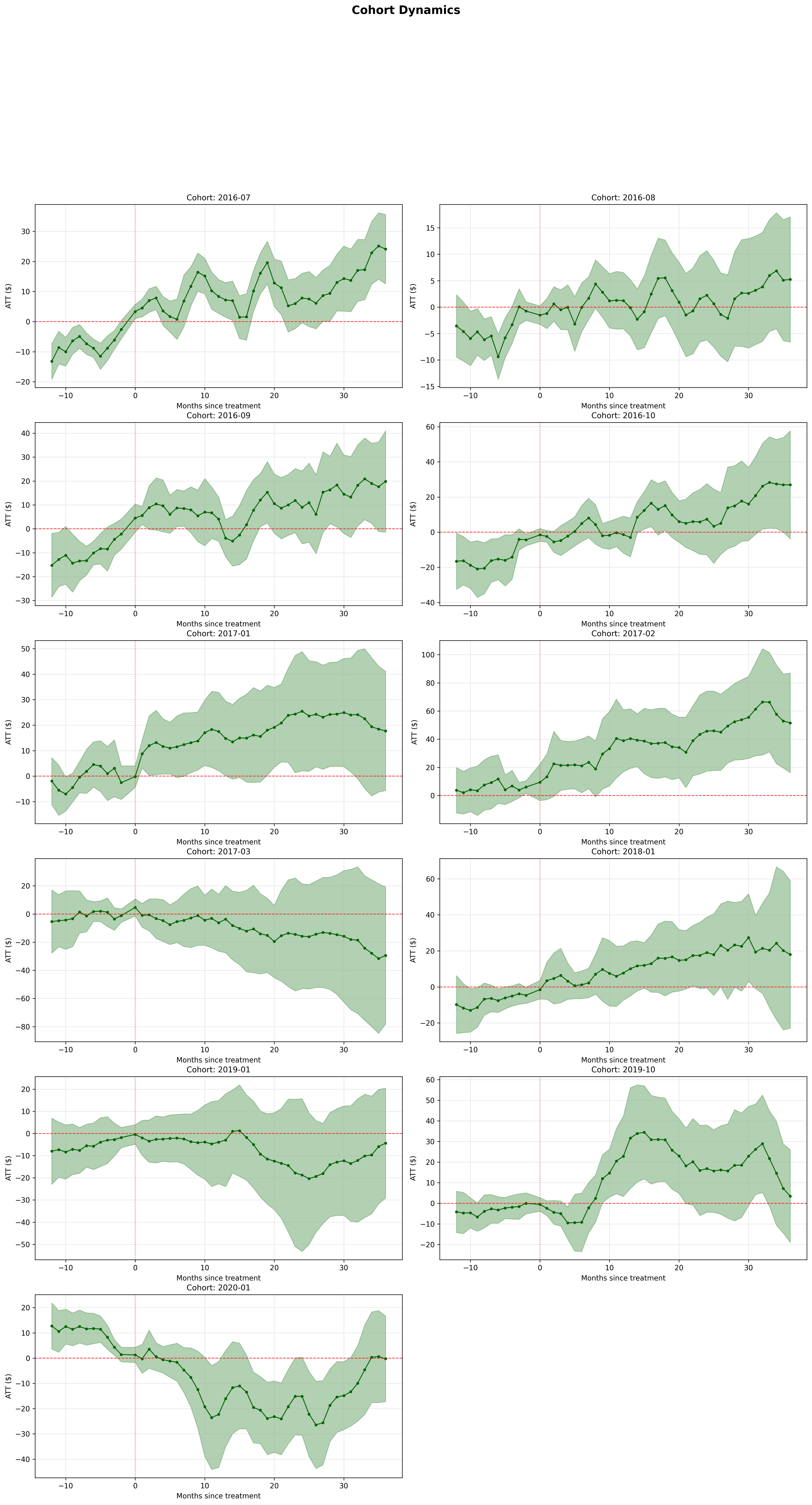
| figures/did_cohort_dynamics.png | Cohort-specific dynamics |
| figures/did_cs_trajectory_fit.png | Post-treatment trajectory (WLS overlays) |
| figures/did_cs_trajectory_phases.png | Early / mid / late phase mean ATTs |
| figures/did_cs_heterogeneity_income.png | Heterogeneity: median income split |
| figures/did_cs_heterogeneity_renter_share.png | Heterogeneity: renter share split |
| figures/did_cs_heterogeneity_airbnb_density.png | Heterogeneity: Airbnb density split |
| figures/did_cs_heterogeneity_dose.png | Heterogeneity: prohibition dose split |
| figures/did_cs_cohort_early_vs_late.png | Heterogeneity: early vs. late cohort |
| figures/did_cs_spillover_event_study.png | Spillover event study |
| csv/did_twfe_cs_comparison_table.csv | TWFE vs CS comparison (tabular) |
| csv/cs_heterogeneity_summary.csv | All subgroup ATTs (income, renter share, Airbnb, dose, cohort) |
| csv/cs_event_study_tract_bootstrap.csv | Tract-cluster bootstrap by rel_time |
| csv/cs_tract_bootstrap_meta.csv | Bootstrap metadata (reps, overall ATT summary) |
| csv/cs_spillover_summary.csv | Spillover overall ATT |
| csv/cs_trajectory_summary.csv | Trajectory phases + shape-fit summary |
| not archived | output/did-cs/did_panel_data.csv and other diagnostic CSVs — run DiD Makefile targets locally |
A.2 Preferred Specification
- Estimator: Callaway–Sant’Anna (2021), aggregated to event study
- Comparison group: Never-treated (robust to not-yet-treated)
- Treatment definition: Threshold at 25th percentile of prohibited-unit share
- Trend matching: k = 3 nearest neighbors, minimum 6 pre-treatment months
- Panel: Monthly tract-level ZORI rental prices, Cook County, Illinois
- Bootstrap: 1,000 tract-cluster resamples, seed 42